Google Sheets: Flag Items That Are Late or Due Soon (With TODAY)
Quick answer
In your Order or Task list, add a column with this formula: =IF(E2="Delivered", "", IF(F2<TODAY(), "LATE", IF(F2-TODAY()<=1, "Due soon", ""))). It checks if a task is done, then flags it late or due within a day. TODAY() changes every day and needs no editing.
Your order or task list has due dates, but you have to scan each row to find what's urgent. A formula can do that for you — one that reads the dates and flags "LATE" or "Due soon" automatically, and updates every day without you editing it.
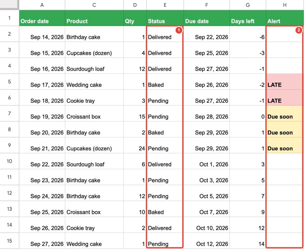
Add the formula
- On your Orders or Tasks tab, add a heading in an empty column (for example H1): Status.
- In the cell below (H2), type this formula exactly:
=IF(E2="Delivered", "", IF(F2<TODAY(), "LATE", IF(F2-TODAY()<=1, "Due soon", ""))) - Press Enter. The cell shows the result for this row.
- Select H2 again, then double-click the small square at its bottom-right corner to copy the formula down to all rows with data.
Free: which spreadsheet problem do you have?
A 6-page PDF: ten everyday Google Sheets problems and the short book that fixes each one.
Get the free overviewWhat the formula does (read it backwards)
The formula has three checks: (1) skip if already delivered, (2) show "LATE" if the due date is before today, (3) show "Due soon" if the due date is within 1 day. Blank if none of those are true.
TODAY() gives today's date and changes every day. When you open the sheet tomorrow, TODAY() updates — no formula editing needed. If the cell shows a date like 1/5/1900, it's just formatting; click the cell and choose Format → Number → Number.
Add color (optional but recommended)
The flags work without color, but red and yellow make them obvious at a glance. Add two conditional formatting rules to the Status column:
- Select the Status column data (for example H2:H15).
- Choose Format → Conditional formatting.
- Under "Format cells if…", choose "Text is exactly". Type LATE and pick a red fill color. Click Done.
- Click the + to add another rule. Choose "Text is exactly" again, type Due soon, pick a yellow fill. Click Done.
One formula isn't a system
Color-coding late items is helpful. It doesn't tell you why they're late — whether the customer didn't reply, you ran out of stock, or someone forgot to deliver. It doesn't show you which customers are waiting most for their orders, or whether late orders are mostly one product.
Those answers come from the whole sheet system: one place to log orders, real dates that work with formulas, dropdowns so names are never typed two ways, and a report that reads the whole list in two formulas. That is what Google Sheets Made Simple builds, one short chapter at a time, using a small bakery's orders and expenses as the example.
Common questions
- Every row shows "LATE" or "Due soon" even though some are still good. Why?
- Check the formula's middle part: F2-TODAY()<=1. This means due-date minus today is 1 or less (so due today or tomorrow). If you see this everywhere, the formula has the comparison backwards or the dates are typed as text.
- The column shows a date like 1/5/1900 instead of "LATE" or "Due soon". Why?
- Google Sheets is formatting the result as a date. Click the cell, then choose Format → Number → Number to see the text properly.
- Can I change when "Due soon" shows? Right now it's 1 day, but I want 3 days.
- Yes. In the formula, change the 1 to 3: IF(F2-TODAY()<=3, "Due soon", ""). Any number of days works.